- How to set up an Excel pivot table.
- How to use calculated metrics in a pivot table.
- How to use Named Ranges in Excel.
- How to use the OFFSET formula in Excel.
Transformation (The “T” in “DTP”)
We are going to use an Excel pivot table for our “transformation” layer in our DTP framework (worksheet). You should already have your data prepared in the “current” worksheet, so you will need to:
1.If you haven’t already, format your data as a table in Excel by highlighting your entire data set in the “current” worksheet and click on “Format as Table” from the “Home” menu.
2.Now select any cell within your table and navigate to the “Insert” menu and insert a “Pivot Table”.
3.Place “Campaign” in the “Report Filter” and “Day” in the “Row Labels” section.
4.Add all metrics to the “Values” section as shown below.
The first calculated metric we are going to create is our “weighted average position” using the “Curr_AvgPos*Impr” metric that we added during our data preparation.
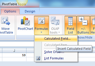
1. Navigate to the “Options” tab in the “PivotTable Tools” menu.
2.Then choose “Calculated Field” from the “Formulas” dropdown.
3.Name your new metric something appropriate like, “AvgPos” and use the following formula: =’Curr_AvgPos*Impr’ /Impressions
4.Repeat steps 1-3 to calculate your previous average position.
Here is a list of the remaining calculated metrics you will need to create using the method described above:
- curr_CTR: =Clicks /Impressions
- curr_CR: =’Conv. (1-per-click)’ /Clicks
- curr_CPC: =Cost /Clicks
- curr_CPA: =Cost /’Conv. (1-per-click)’
- prv_CTR: =Prv_Clicks /Prv_Impr
- prv_CR: =Prv_Conv /Prv_Clicks
- prv_CPC: =Prv_Cost /Prv_Clicks
- prv_CPA: =Prv_Cost /Prv_Conv
Here is a list of all the columns you should now have in your pivot table:
| Row Labels |
| Sum of Impressions |
| Sum of Clicks |
| Sum of Cost |
| Sum of Conv. (1-per-click) |
| Sum of AvgPos |
| Sum of Prv_Impr |
| Sum of Prv_Clicks |
| Sum of Prv_Cost |
| Sum of Prv_Conv |
| Sum of Prv_AvgPos |
| Sum of curr_CTR |
| Sum of curr_CR |
| Sum of curr_CPC |
| Sum of curr_CPA |
| Sum of prv_CTR |
| Sum of prv_CR |
| Sum of prv_CPC |
| Sum of prv_CPA |
| Sum of Curr_AvgPos*Impr |
| Sum of Prv_AvgPos*Impr |
In order for our dashboard to be dynamic we will need to “Define Names” for all of the columns in our pivot table. We will also be using the OFFSET formula to allow for the selecting of different date ranges like in the AdWords dashboard we are re-creating.
Let’s start with “date”.
1.Navigate to the “Formulas” ribbon and select “Define Name” from the menu.
2. Use “date” for the name and the following formula in the “Refers to:” field: =OFFSET(transform!$A$5, transform!$J$1, 0, transform!$K$1+1,1)
Now that we’ve defined our left-most column, “date”, we can use the OFFSET formula to define the remaining columns.
3. Follow the steps above to get back to define a new name and use the name “curr_impr” and the following formula: =OFFSET(date,0,1)
4. Continue to define the names of your columns and increment your OFFSET formula using the “date” named range as seen below:
Next we are going to work on our “presentation” layer. This will include our charts and summaries as well as the dynamic controls we will need to manipulate date-ranges and campaigns.
by Chad Summerhill, author of the blog PPC Prospector, provider of free PPC tools and PPC tutorials, and in-house AdWords Specialist at Moving Solutions, Inc. (UPack.com and MoveBuilder.com).
(Learn More Excel Tips: Excel Bubble Chart Tutorial)


0 Comments